11.2. 注意力汇聚：Nadaraya-Watson 核回归

在 Colab 中打开 [pytorch]

在 Colab 中打开 Notebook

在 Colab 中打开 [mxnet]

在 Colab 中打开 Notebook

在 Colab 中打开 [jax]

在 Colab 中打开 Notebook

在 Colab 中打开 [tensorflow]

在 Colab 中打开 Notebook

在 SageMaker Studio Lab 中打开

在 SageMaker Studio Lab 中打开 Notebook

现在我们已经介绍了注意力机制的主要组成部分，让我们在一个相当经典的设置下使用它们，即通过核密度估计进行回归和分类 (Nadaraya, 1964, Watson, 1964)。这部分内容只是提供额外的背景知识：它完全是可选的，如果需要可以跳过。Nadaraya-Watson估计器的核心依赖于某个将查询 \(\mathbf{q}\) 和键 \(\mathbf{k}\) 关联起来的相似性核 \(\alpha(\mathbf{q}, \mathbf{k})\)。一些常见的核函数如下：

(11.2.1)\[\begin{split}\begin{aligned} \alpha(\mathbf{q}, \mathbf{k}) & = \exp\left(-\frac{1}{2} \|\mathbf{q} - \mathbf{k}\|^2 \right) && \textrm{高斯核 (Gaussian);} \\ \alpha(\mathbf{q}, \mathbf{k}) & = 1 \textrm{ if } \|\mathbf{q} - \mathbf{k}\| \leq 1 && \textrm{箱形核 (Boxcar);} \\ \alpha(\mathbf{q}, \mathbf{k}) & = \mathop{\mathrm{max}}\left(0, 1 - \|\mathbf{q} - \mathbf{k}\|\right) && \textrm{Epanechikov核.} \end{aligned}\end{split}\]

我们还可以选择更多的核函数。可以参阅 维基百科文章 以获得更广泛的评论，以及核函数的选择如何与核密度估计（有时也称为 *Parzen 窗* (Parzen, 1957)）相关联。所有这些核函数都是启发式的，并且可以进行调整。例如，我们不仅可以在全局范围内调整宽度，甚至可以在每个坐标上进行调整。无论如何，它们都导致了以下适用于回归和分类的方程：

(11.2.2)\[f(\mathbf{q}) = \sum_i \mathbf{v}_i \frac{\alpha(\mathbf{q}, \mathbf{k}_i)}{\sum_j \alpha(\mathbf{q}, \mathbf{k}_j)}.\]

对于一个（标量）回归问题，观测值为 \((\mathbf{x}_i, y_i)\)，分别代表特征和标签，其中 \(\mathbf{v}_i = y_i\) 是标量，\(\mathbf{k}_i = \mathbf{x}_i\) 是向量，查询 \(\mathbf{q}\) 表示需要评估 \(f\) 的新位置。在（多类）分类的情况下，我们使用 \(y_i\) 的独热编码来获得 \(\mathbf{v}_i\)。这种估计器的一个便利特性是它不需要训练。更进一步，如果我们随着数据量的增加适当地缩小核的宽度，该方法是一致的 (Mack and Silverman, 1982)，也就是说，它将收敛到某个统计上最优的解。让我们从检查一些核函数开始。

pytorchmxnetjaxtensorflow

import numpy as np
import torch
from torch import nn
from torch.nn import functional as F
from d2l import torch as d2l

d2l.use_svg_display()

from mxnet import autograd, gluon, np, npx
from mxnet.gluon import nn
from d2l import mxnet as d2l

npx.set_np()
d2l.use_svg_display()

import jax
from flax import linen as nn
from jax import numpy as jnp
from d2l import jax as d2l

No GPU/TPU found, falling back to CPU. (Set TF_CPP_MIN_LOG_LEVEL=0 and rerun for more info.)

import numpy as np
import tensorflow as tf
from d2l import tensorflow as d2l

d2l.use_svg_display()

11.2.1. 核函数和数据

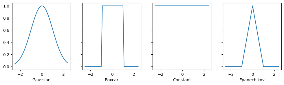
本节中定义的所有核函数 \(\alpha(\mathbf{k}, \mathbf{q})\) 都是*平移和旋转不变的*；也就是说，如果我们以相同的方式平移和旋转 \(\mathbf{k}\) 和 \(\mathbf{q}\)，\(\alpha\) 的值保持不变。为简单起见，我们因此选择标量参数 \(k, q \in \mathbb{R}\) 并选择键 \(k = 0\) 作为原点。这得到：

pytorchmxnetjaxtensorflow

# Define some kernels
def gaussian(x):
    return torch.exp(-x**2 / 2)

def boxcar(x):
    return torch.abs(x) < 1.0

def constant(x):
    return 1.0 + 0 * x

def epanechikov(x):
    return torch.max(1 - torch.abs(x), torch.zeros_like(x))

fig, axes = d2l.plt.subplots(1, 4, sharey=True, figsize=(12, 3))

kernels = (gaussian, boxcar, constant, epanechikov)
names = ('Gaussian', 'Boxcar', 'Constant', 'Epanechikov')
x = torch.arange(-2.5, 2.5, 0.1)
for kernel, name, ax in zip(kernels, names, axes):
    ax.plot(x.detach().numpy(), kernel(x).detach().numpy())
    ax.set_xlabel(name)

d2l.plt.show()

# Define some kernels
def gaussian(x):
    return np.exp(-x**2 / 2)

def boxcar(x):
    return np.abs(x) < 1.0

def constant(x):
    return 1.0 + 0 * x

def epanechikov(x):
    return np.maximum(1 - np.abs(x), 0)

fig, axes = d2l.plt.subplots(1, 4, sharey=True, figsize=(12, 3))

kernels = (gaussian, boxcar, constant, epanechikov)
names = ('Gaussian', 'Boxcar', 'Constant', 'Epanechikov')
x = np.arange(-2.5, 2.5, 0.1)
for kernel, name, ax in zip(kernels, names, axes):
    ax.plot(x.asnumpy(), kernel(x).asnumpy())
    ax.set_xlabel(name)

d2l.plt.show()

[22:04:09] ../src/storage/storage.cc:196: Using Pooled (Naive) StorageManager for CPU

# Define some kernels
def gaussian(x):
    return jnp.exp(-x**2 / 2)

def boxcar(x):
    return jnp.abs(x) < 1.0

def constant(x):
    return 1.0 + 0 * x

def epanechikov(x):
    return jnp.maximum(1 - jnp.abs(x), 0)

fig, axes = d2l.plt.subplots(1, 4, sharey=True, figsize=(12, 3))

kernels = (gaussian, boxcar, constant, epanechikov)
names = ('Gaussian', 'Boxcar', 'Constant', 'Epanechikov')
x = jnp.arange(-2.5, 2.5, 0.1)
for kernel, name, ax in zip(kernels, names, axes):
    ax.plot(x, kernel(x))
    ax.set_xlabel(name)

d2l.plt.show()

# Define some kernels
def gaussian(x):
    return tf.exp(-x**2 / 2)

def boxcar(x):
    return tf.abs(x) < 1.0

def constant(x):
    return 1.0 + 0 * x

def epanechikov(x):
    return tf.maximum(1 - tf.abs(x), 0)

fig, axes = d2l.plt.subplots(1, 4, sharey=True, figsize=(12, 3))

kernels = (gaussian, boxcar, constant, epanechikov)
names = ('Gaussian', 'Boxcar', 'Constant', 'Epanechikov')
x = tf.range(-2.5, 2.5, 0.1)
for kernel, name, ax in zip(kernels, names, axes):
    ax.plot(x.numpy(), kernel(x).numpy())
    ax.set_xlabel(name)

d2l.plt.show()

不同的核函数对应于不同的范围和平滑度概念。例如，箱形核只关注距离在 \(1\) （或其他定义的超参数）之内的观测值，并且无差别地对待它们。

为了观察 Nadaraya-Watson 估计的实际效果，让我们定义一些训练数据。在下文中，我们使用以下依赖关系：

(11.2.3)\[y_i = 2\sin(x_i) + x_i + \epsilon,\]

其中 \(\epsilon\) 从零均值和单位方差的正态分布中抽取。我们抽取 40 个训练样本。

pytorchmxnetjaxtensorflow

def f(x):
    return 2 * torch.sin(x) + x

n = 40
x_train, _ = torch.sort(torch.rand(n) * 5)
y_train = f(x_train) + torch.randn(n)
x_val = torch.arange(0, 5, 0.1)
y_val = f(x_val)

def f(x):
    return 2 * np.sin(x) + x

n = 40
x_train = np.sort(np.random.rand(n) * 5, axis=None)
y_train = f(x_train) + np.random.randn(n)
x_val = np.arange(0, 5, 0.1)
y_val = f(x_val)

def f(x):
    return 2 * jnp.sin(x) + x

n = 40
x_train = jnp.sort(jax.random.uniform(d2l.get_key(), (n,)) * 5)
y_train = f(x_train) + jax.random.normal(d2l.get_key(), (n,))
x_val = jnp.arange(0, 5, 0.1)
y_val = f(x_val)

def f(x):
    return 2 * tf.sin(x) + x

n = 40
x_train = tf.sort(tf.random.uniform((n,1)) * 5, 0)
y_train = f(x_train) + tf.random.normal((n, 1))
x_val = tf.range(0, 5, 0.1)
y_val = f(x_val)

11.2.2. 通过 Nadaraya-Watson 回归实现注意力汇聚

现在我们有了数据和核函数，我们只需要一个计算核回归估计的函数。请注意，我们还希望获得相对核权重，以便进行一些简单的诊断。因此，我们首先计算所有训练特征（协变量）x_train 和所有验证特征 x_val 之间的核。这会产生一个矩阵，我们随后对其进行归一化。当与训练标签 y_train 相乘时，我们得到估计值。

回顾 (11.1.1) 中的注意力汇聚。让每个验证特征作为查询，每个训练特征-标签对作为键值对。因此，归一化后的相对核权重（下面的 attention_w）就是*注意力权重*。

pytorchmxnetjaxtensorflow

def nadaraya_watson(x_train, y_train, x_val, kernel):
    dists = x_train.reshape((-1, 1)) - x_val.reshape((1, -1))
    # Each column/row corresponds to each query/key
    k = kernel(dists).type(torch.float32)
    # Normalization over keys for each query
    attention_w = k / k.sum(0)
    y_hat = y_train@attention_w
    return y_hat, attention_w

def nadaraya_watson(x_train, y_train, x_val, kernel):
    dists = x_train.reshape((-1, 1)) - x_val.reshape((1, -1))
    # Each column/row corresponds to each query/key
    k = kernel(dists).astype(np.float32)
    # Normalization over keys for each query
    attention_w = k / k.sum(0)
    y_hat = np.dot(y_train, attention_w)
    return y_hat, attention_w

def nadaraya_watson(x_train, y_train, x_val, kernel):
    dists = x_train.reshape((-1, 1)) - x_val.reshape((1, -1))
    # Each column/row corresponds to each query/key
    k = kernel(dists).astype(jnp.float32)
    # Normalization over keys for each query
    attention_w = k / k.sum(0)
    y_hat = y_train@attention_w
    return y_hat, attention_w

def nadaraya_watson(x_train, y_train, x_val, kernel):
    dists = tf.reshape(x_train, (-1, 1)) - tf.reshape(x_val, (1, -1))
    # Each column/row corresponds to each query/key
    k = tf.cast(kernel(dists), tf.float32)
    # Normalization over keys for each query
    attention_w = k / tf.reduce_sum(k, 0)
    y_hat = tf.transpose(tf.transpose(y_train)@attention_w)
    return y_hat, attention_w

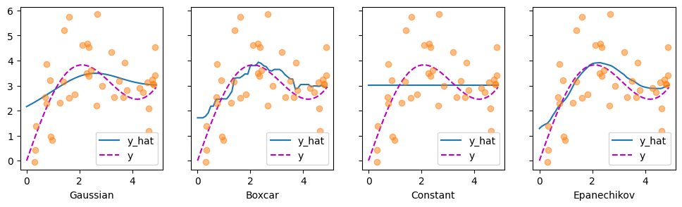
让我们看看不同核函数产生的估计类型。

pytorchmxnetjaxtensorflow

def plot(x_train, y_train, x_val, y_val, kernels, names, attention=False):
    fig, axes = d2l.plt.subplots(1, 4, sharey=True, figsize=(12, 3))
    for kernel, name, ax in zip(kernels, names, axes):
        y_hat, attention_w = nadaraya_watson(x_train, y_train, x_val, kernel)
        if attention:
            pcm = ax.imshow(attention_w.detach().numpy(), cmap='Reds')
        else:
            ax.plot(x_val, y_hat)
            ax.plot(x_val, y_val, 'm--')
            ax.plot(x_train, y_train, 'o', alpha=0.5);
        ax.set_xlabel(name)
        if not attention:
            ax.legend(['y_hat', 'y'])
    if attention:
        fig.colorbar(pcm, ax=axes, shrink=0.7)

plot(x_train, y_train, x_val, y_val, kernels, names)

def plot(x_train, y_train, x_val, y_val, kernels, names, attention=False):
    fig, axes = d2l.plt.subplots(1, 4, sharey=True, figsize=(12, 3))
    for kernel, name, ax in zip(kernels, names, axes):
        y_hat, attention_w = nadaraya_watson(x_train, y_train, x_val, kernel)
        if attention:
            pcm = ax.imshow(attention_w.asnumpy(), cmap='Reds')
        else:
            ax.plot(x_val, y_hat)
            ax.plot(x_val, y_val, 'm--')
            ax.plot(x_train, y_train, 'o', alpha=0.5);
        ax.set_xlabel(name)
        if not attention:
            ax.legend(['y_hat', 'y'])
    if attention:
        fig.colorbar(pcm, ax=axes, shrink=0.7)

plot(x_train, y_train, x_val, y_val, kernels, names)

def plot(x_train, y_train, x_val, y_val, kernels, names, attention=False):
    fig, axes = d2l.plt.subplots(1, 4, sharey=True, figsize=(12, 3))
    for kernel, name, ax in zip(kernels, names, axes):
        y_hat, attention_w = nadaraya_watson(x_train, y_train, x_val, kernel)
        if attention:
            pcm = ax.imshow(attention_w, cmap='Reds')
        else:
            ax.plot(x_val, y_hat)
            ax.plot(x_val, y_val, 'm--')
            ax.plot(x_train, y_train, 'o', alpha=0.5);
        ax.set_xlabel(name)
        if not attention:
            ax.legend(['y_hat', 'y'])
    if attention:
        fig.colorbar(pcm, ax=axes, shrink=0.7)

plot(x_train, y_train, x_val, y_val, kernels, names)

def plot(x_train, y_train, x_val, y_val, kernels, names, attention=False):
    fig, axes = d2l.plt.subplots(1, 4, sharey=True, figsize=(12, 3))
    for kernel, name, ax in zip(kernels, names, axes):
        y_hat, attention_w = nadaraya_watson(x_train, y_train, x_val, kernel)
        if attention:
            pcm = ax.imshow(attention_w.numpy(), cmap='Reds')
        else:
            ax.plot(x_val, y_hat)
            ax.plot(x_val, y_val, 'm--')
            ax.plot(x_train, y_train, 'o', alpha=0.5);
        ax.set_xlabel(name)
        if not attention:
            ax.legend(['y_hat', 'y'])
    if attention:
        fig.colorbar(pcm, ax=axes, shrink=0.7)

plot(x_train, y_train, x_val, y_val, kernels, names)

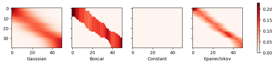
首先引人注目的是，所有三个非平凡核（高斯核、箱形核和 Epanechikov 核）都产生了相当可行的估计，与真实函数相差不远。只有常数核导致了平凡的估计 \(f(x) = \frac{1}{n} \sum_i y_i\)，产生了相当不切实际的结果。让我们更仔细地检查一下注意力权重。

pytorchmxnetjaxtensorflow

plot(x_train, y_train, x_val, y_val, kernels, names, attention=True)

plot(x_train, y_train, x_val, y_val, kernels, names, attention=True)

plot(x_train, y_train, x_val, y_val, kernels, names, attention=True)

plot(x_train, y_train, x_val, y_val, kernels, names, attention=True)

可视化清楚地显示了为什么高斯核、箱形核和 Epanechikov 核的估计非常相似：毕竟，它们是从非常相似的注意力权重中得出的，尽管核的函数形式不同。这就提出了一个问题，即这种情况是否总是如此。

11.2.3. 自适应注意力汇聚

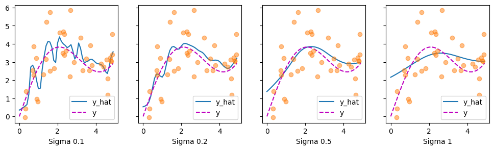
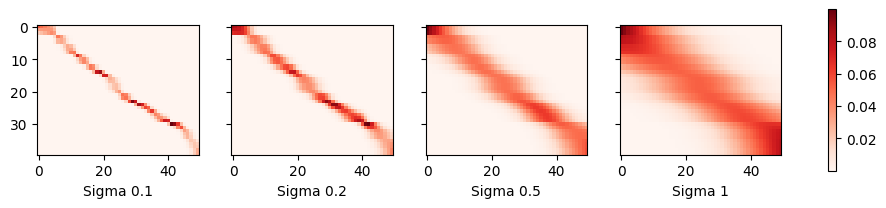
我们可以用不同宽度的高斯核来替换。也就是说，我们可以使用 \(\alpha(\mathbf{q}, \mathbf{k}) = \exp\left(-\frac{1}{2 \sigma^2} \|\mathbf{q} - \mathbf{k}\|^2 \right)\)，其中 \(\sigma^2\) 决定了核的宽度。让我们看看这是否会影响结果。

pytorchmxnetjaxtensorflow

sigmas = (0.1, 0.2, 0.5, 1)
names = ['Sigma ' + str(sigma) for sigma in sigmas]

def gaussian_with_width(sigma):
    return (lambda x: torch.exp(-x**2 / (2*sigma**2)))

kernels = [gaussian_with_width(sigma) for sigma in sigmas]
plot(x_train, y_train, x_val, y_val, kernels, names)

sigmas = (0.1, 0.2, 0.5, 1)
names = ['Sigma ' + str(sigma) for sigma in sigmas]

def gaussian_with_width(sigma):
    return (lambda x: np.exp(-x**2 / (2*sigma**2)))

kernels = [gaussian_with_width(sigma) for sigma in sigmas]
plot(x_train, y_train, x_val, y_val, kernels, names)

sigmas = (0.1, 0.2, 0.5, 1)
names = ['Sigma ' + str(sigma) for sigma in sigmas]

def gaussian_with_width(sigma):
    return (lambda x: jnp.exp(-x**2 / (2*sigma**2)))

kernels = [gaussian_with_width(sigma) for sigma in sigmas]
plot(x_train, y_train, x_val, y_val, kernels, names)

sigmas = (0.1, 0.2, 0.5, 1)
names = ['Sigma ' + str(sigma) for sigma in sigmas]

def gaussian_with_width(sigma):
    return (lambda x: tf.exp(-x**2 / (2*sigma**2)))

kernels = [gaussian_with_width(sigma) for sigma in sigmas]
plot(x_train, y_train, x_val, y_val, kernels, names)

显然，核越窄，估计就越不平滑。同时，它能更好地适应局部变化。让我们看看相应的注意力权重。

pytorchmxnetjaxtensorflow

plot(x_train, y_train, x_val, y_val, kernels, names, attention=True)

plot(x_train, y_train, x_val, y_val, kernels, names, attention=True)

plot(x_train, y_train, x_val, y_val, kernels, names, attention=True)

plot(x_train, y_train, x_val, y_val, kernels, names, attention=True)

正如我们所预料的，核越窄，大注意力权重的范围就越窄。同样清楚的是，选择相同的宽度可能并不理想。事实上，Silverman (1986) 提出了一个依赖于局部密度的启发式方法。还有许多类似的“技巧”被提出。例如，Norelli 等人 (2022) 使用了一种类似的最近邻插值技术来设计跨模态的图像和文本表示。

敏锐的读者可能会想，我们为什么要对一个已有半个多世纪历史的方法进行如此深入的探讨。首先，它是现代注意力机制的最早先驱之一。其次，它非常适合可视化。第三，同样重要的是，它展示了手工制作的注意力机制的局限性。一个更好的策略是*学习*这个机制，通过学习查询和键的表示。这正是我们将在以下章节中开始探讨的。

11.2.4. 小结

Nadaraya-Watson 核回归是当前注意力机制的早期先驱。它几乎不需要训练或调整就可以直接用于分类或回归。注意力权重根据查询和键之间的相似度（或距离）以及可用的相似观测值的数量来分配。

11.2.5. 练习

1. Parzen 窗密度估计由 \(\hat{p}(\mathbf{x}) = \frac{1}{n} \sum_i k(\mathbf{x}, \mathbf{x}_i)\) 给出。证明对于二元分类，通过 Parzen 窗得到的函数 \(\hat{p}(\mathbf{x}, y=1) - \hat{p}(\mathbf{x}, y=-1)\) 等价于 Nadaraya-Watson 分类。

2. 实现随机梯度下降来学习 Nadaraya-Watson 回归中核宽度的良好值。

   1. 如果直接使用上述估计来最小化 \((f(\mathbf{x_i}) - y_i)^2\) 会发生什么？提示：\(y_i\) 是用于计算 \(f\) 的项的一部分。

   2. 从 \(f(\mathbf{x}_i)\) 的估计中移除 \((\mathbf{x}_i, y_i)\)，并对核宽度进行优化。你是否仍然观察到过拟合？

3. 假设所有的 \(\mathbf{x}\) 都在单位球面上，即都满足 \(\|\mathbf{x}\| = 1\)。你能简化指数项中的 \(\|\mathbf{x} - \mathbf{x}_i\|^2\) 吗？提示：我们稍后会看到这与点积注意力非常相关。

4. 回想一下，Mack 和 Silverman (1982) 证明了 Nadaraya-Watson 估计是一致的。随着数据量的增加，你应该多快地减小注意力机制的尺度？为你的答案提供一些直觉。它是否依赖于数据的维度？如何依赖？

pytorchmxnetjaxtensorflow

讨论

讨论

讨论

讨论